VGG16 Fine-tuning model

Overview

On the article, VGG19 Fine-tuning model, I checked VGG19’s architecture and made fine-tuning model. On the same way, I’ll show the architecture VGG16 and make model here.

There are some image classification models we can use for fine-tuning.
Those model's weights are already trained and by small steps, you can make models for your own data.

About the fine-tuning itself, please check the followings.

• How to make Fine tuning model by Keras
• VGG19 Fine-tuning model

VGG16

As preparation, you need to install necessary libraries by following commands.

pip install pydot graphviz
pip install pydot3 pydot-ng

By executing folloing code, we can visualize the VGG16 model’s architecture.

from IPython.display import SVG
from keras.applications.vgg16 import VGG16
from keras.utils.vis_utils import model_to_dot
vgg_model = VGG16(weights='imagenet', include_top=False)
SVG(model_to_dot(vgg_model).create(prog='dot', format='svg'))

The model is composed of convolutional and pooling layers. You can say this has very simple architecture.
For fine-tuning, we need to choose re-train target layers. Naively, we can check layer’s numbers and names.

# check the layers by name
for i,layer in enumerate(vgg_model.layers):
    print(i,layer.name)

0 input_3
1 block1_conv1
2 block1_conv2
3 block1_pool
4 block2_conv1
5 block2_conv2
6 block2_pool
7 block3_conv1
8 block3_conv2
9 block3_conv3
10 block3_pool
11 block4_conv1
12 block4_conv2
13 block4_conv3
14 block4_pool
15 block5_conv1
16 block5_conv2
17 block5_conv3
18 block5_pool

Data

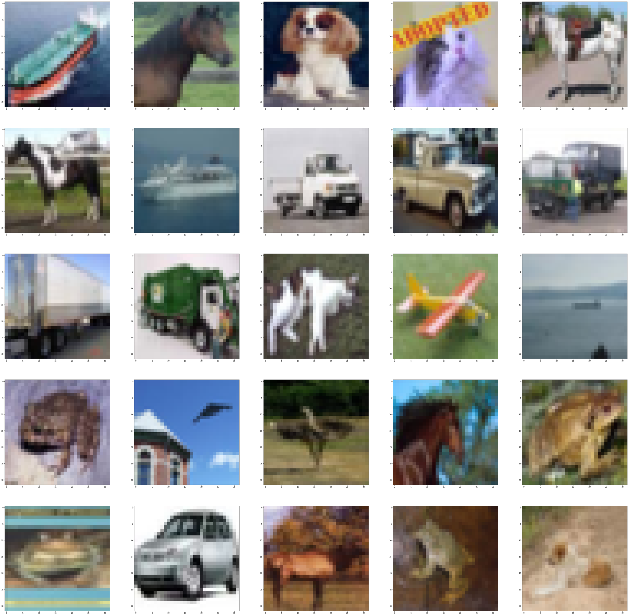
Same as the article, VGG19 Fine-tuning model, I used cifar-10, simple color image data set.
This time, for fine-tuning, I limited the amount of data for training and size.

import random
import cv2
from keras.datasets import cifar10
from keras.utils import to_categorical
from keras.models import Model
from keras.layers import Dense, GlobalAveragePooling2D, Dropout
from keras.optimizers import SGD
import numpy as np

# read data
(x_train, y_train), (x_test, y_test) = cifar10.load_data()

# limit the amount of the data
# train data
ind_train = random.sample(list(range(x_train.shape[0])), 2000)
x_train = x_train[ind_train]
y_train = y_train[ind_train]

# test data
ind_test = random.sample(list(range(x_test.shape[0])), 2000)
x_test = x_test[ind_test]
y_test = y_test[ind_test]

def resize_data(data):
    data_upscaled = np.zeros((data.shape[0], 48, 48, 3))
    for i, img in enumerate(data):
        large_img = cv2.resize(img, dsize=(48, 48), interpolation=cv2.INTER_CUBIC)
        data_upscaled[i] = large_img

    return data_upscaled

# resize train and  test data
x_train_resized = resize_data(x_train)
x_test_resized = resize_data(x_test)

# make explained variable hot-encoded
y_train_hot_encoded = to_categorical(y_train)
y_test_hot_encoded = to_categorical(y_test)

Fine-tuning

Here, I added fully connected layers, selected training target layers, and trained.
About the detail about the things done on this point, please check the article below.

• How to make Fine tuning model by Keras

# get layers and add average pooling layer
x = vgg_model.output
x = GlobalAveragePooling2D()(x)

# add fully-connected layer
x = Dense(512, activation='relu')(x)
x = Dropout(0.3)(x)

# add output layer
predictions = Dense(10, activation='softmax')(x)

model = Model(inputs=vgg_model.input, outputs=predictions)

# freeze pre-trained model area's layer
for layer in vgg_model.layers:
    layer.trainable = False

# update the weight that are added
model.compile(optimizer='rmsprop', loss='categorical_crossentropy')
model.fit(x_train_resized, y_train_hot_encoded)

# choose the layers which are updated by training
layer_num = len(model.layers)
for layer in model.layers[:18]:
    layer.trainable = False

for layer in model.layers[18:]:
    layer.trainable = True

# training
model.compile(optimizer=SGD(lr=0.0001, momentum=0.9), loss='categorical_crossentropy', metrics=['accuracy'])
history = model.fit(x_train_resized, y_train_hot_encoded, batch_size=256, epochs=50, shuffle=True,  validation_split=0.1)

To check how train went on, we can get the plot.

import matplotlib.pyplot as plt
def show_history(history):
    plt.plot(history.history['acc'])
    plt.plot(history.history['val_acc'])
    plt.ylabel('accuracy')
    plt.xlabel('epoch')
    plt.legend(['train_accuracy', 'test_accuracy'], loc='best')
    plt.show()

show_history(history)