Abstract
This article covers basic understanding and coding of Residual module. If you have experience of using fine tuning or frequently tackle with image recognition tasks, probably you have heard the network name, ResNet. ResNet is composed of Residual module, whose structure is expressed as below.The image above is from https://arxiv.org/abs/1512.03385.
Basically, deeper neural network contributes to the better outcome. If you have enough computational resource(unfortunately, I don't have), for difficult task, you can approach it with really deep neural network. However, with deeper neural network, the problem of degradation comes, which makes it difficult to train the model. Residual module offers one of the solutions to this problem, meaning that with this, we can make deeper neural network by softening the difficulty of training.
For precise and better understanding, I recommend that you read the paper below. Here, I'll just show summary for simple and concise understanding and coding with Keras.
If there are strange or wrong points, please let me know by comment or message.
Residual module
Structure of Convolutional Neural Network
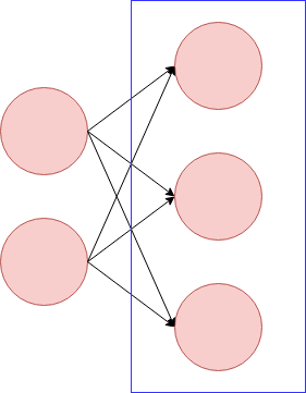
Before tackling with Residual module, I'll roughly touch the structure of CNN(Convolutional Neural Network) itself. CNN is composed of convolutional layer and dense layer, although to say precisely input, output layers and pooling layers should be added. And about network architecture, we need to care about the number of layers and nodes.
On the image above, the red circles express the nodes. The blue rectangle expresses one layer. When we make CNN model, we need to think about those of convolutional and dense layer.
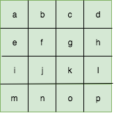
From here, let’s focus on convolutional layer. Assume there is an image like below. The height and width are four.

When we adapt convolution to this, we will choose the kernel size. The example below is the kernel with the size (3, 3) with stride (1,1).

On the context of convolutional neural network, the parameters w1 ~ w9 are the targets to update.
As you can see, by the size of kernel, the outcome of the convolutional network changes.
Residual module
The point of Residual module is the identity mapping. On the image below, the input to the module, , is added to the output. This is the characteristics of Residual module.
The image above is from https://arxiv.org/abs/1512.03385.
Concept of Residual module
As I wrote above, when we make a convolutional neural network, we need to care about the layers and nodes of convolutional and dense layers. Residual module will soften the problem caused by increasing the number of layers. When we make a neural network, there are some typical problems as following.- vanishing gradients
- exploding gradients
- degradation
When deeper networks are able to start converging, a degradation problem has been exposed: with the network depth increasing, accuracy gets saturated (which might be unsurprising) and then degrades rapidly. Unexpectedly, such degradation is not caused by overfitting, and adding more layers to a suitably deep model leads to higher train- ing error, as reported in [11, 42] and thoroughly verified by our experiments. Fig. 1 shows a typical example.
This can be obstacle to make deeper neural network. Residual module try to soften this problem and help to increase the number of layers.
Code
From here, I'll write two types of Residual modules and by embedding those make models. Keras enables us to write those relatively easily.As the training data set, I'll use MNIST dataset.
At first, import necessary libraries and load MNIST dataset. The purpose of this article is to show Residual module. So, here I will use just 2000 for training.
from keras.datasets import mnist
from keras.utils import to_categorical

(x_train, y_train), (x_test, y_test) = mnist.load_data()

x_train = x_train.reshape((60000, 28, 28, 1))[0:2000]
y_train = to_categorical(y_train, 10)[0:2000]
The code below is to make the Residual module. This has two convolutional layers with batch normalization. On the last part of the module, the input to the module is added. This function doesn't work if the input’s channel is not equal to 1, because on
output = Add()([h_2, inputs]), the inputs is added to h_2 by broadcasting. import keras
from keras.layers import Conv2D, Dense, BatchNormalization, ReLU, Add, Input, Flatten
from keras.models import Model
def residual_a(inputs):
h_1 = Conv2D(6, (3,3), border_mode='same')(inputs)
h_1 = BatchNormalization()(h_1)
h_1 = ReLU()(h_1)
h_2 = Conv2D(6, (3,3), border_mode='same')(h_1)
h_2 = BatchNormalization()(h_2)
output = Add()([h_2, inputs])
return output
This is expressed by the following image which is quoted by https://arxiv.org/abs/1512.03385.

By using this module(function), I'll make a simple model. The advantage of residual module is related with the depth of the network. This will prevent from degradation on deeper networks. So, I should make very deep network to check the effect. But, my computational resource is not enough to do that and I'm reluctant to rent a server just for this experiment even by getting wife's anger. Because of this, I'll make really simple and shallow network.
def residual_model_a(x_train):

    inputs = Input(x_train.shape[1:])

    x = residual_a(inputs)
    x = Flatten()(x)
    x = Dense(64, activation='relu')(x)
    predictions = Dense(10, activation='softmax')(x)

    model = Model(input=inputs, output=predictions)

    model.compile(loss=keras.losses.categorical_crossentropy,
                 optimizer=keras.optimizers.SGD(lr=0.0001),
                 metrics=['accuracy'])
    return model
By using MNIST data set, the following code block will train the model and show the outcome with visualization.
%matplotlib inline
import matplotlib.pyplot as plt

model_a = residual_model_a(x_train)
model_a.fit(x_train, y_train, epochs=50, shuffle=True, validation_split=0.1)

def show_history(history):
    plt.plot(history.history['acc'])
    plt.plot(history.history['val_acc'])
    plt.ylabel('accuracy')
    plt.xlabel('epoch')
    plt.legend(['train_accuracy', 'test_accuracy'], loc='best')
    plt.show()

show_history(model_a.history)

Also, we can use 1x1 Conv2D mapping for shortcut. The difference between and is the shortcut part. Although on the is added as it is, on the go through the Conv2D with 1x1 kernel size.
def residual_b(inputs):

    h_1 = Conv2D(6, (3,3), border_mode='same')(inputs)
    h_1 = BatchNormalization()(h_1)
    h_1 = ReLU()(h_1)

    h_2 = Conv2D(6, (3,3), border_mode='same')(h_1)
    h_2 = BatchNormalization()(h_2)

    shortcut = Conv2D(6, (1,1), padding='same')(inputs)
    shortcut = BatchNormalization()(shortcut)

    output = Add()([h_2, shortcut])
    return output

def residual_model_b(x_train):

    inputs = Input(x_train.shape[1:])

    x = residual_b(inputs)
    x = Flatten()(x)
    x = Dense(64, activation='relu')(x)
    predictions = Dense(10, activation='softmax')(x)

    model = Model(input=inputs, output=predictions)

    model.compile(loss=keras.losses.categorical_crossentropy,
                 optimizer=keras.optimizers.SGD(lr=0.0001),
                 metrics=['accuracy'])
    return model

model_b = residual_model_b(x_train)
model_b.fit(x_train, y_train, epochs=50, shuffle=True, validation_split=0.1)
show_history(model_b.history)
