Probabilistic Clustering with EM algorithm: Algorithm and Visualization with Julia from scratch

Abstract

On this article, I'll write probabilistic clustering by EM algorithm from scratch with Julia. Here, I'll touch only about mixture of Gaussian case.
The outcome of clustering becomes below. To the simple artificial data, it is working.

Probabilistic Clustering

On the clustering by probabilistic model, the probabilistic models are applied on the data distribution and on probabilistic way, the clusters the data belong to can be chosen.
On hard clustering like K-means, the outcome becomes like below.

a	b
1	0
0	1
1	0

On this case, there are three data points and the first and third ones belong to the cluster a and the second one belongs to cluster b.
From the viewpoint of consequence, on the clustering by probabilistic model, it becomes as below.

a	b
0.8	0.2
0.4	0.6
0.9	0.1

As an outcome, probabilities are really informative.
But what we should pay attention on is not the form of outcome but the system of probabilistic modeling. Roughly, the system is as followings.

• regard the data as being generated by the probabilistic model
• estimate the probabilistic model's parameters

This is simple but strong and consistent approach in various situations. The theme of this article is clustering. So, by using that as example, let's trace the system.

When we do clustering, the number of clusters is more than one. To express the whole probability distributions, we can set the linear combination of some probabilistic models.

On this article, I'll use normal distribution as the probabilistic model. On this case, we can express the whole probability distribution as following.
$p(x) = \sum_{k=1}^{K}\pi_k\mathcal{N(x|\mu_k, \Sigma_k)}$
The $x$ means the data and the $\pi_k$ means the mixing ratio. For now, there are three parameters to estimate, $\pi_k$, $\mu_k$ and $\Sigma_k$. To think about those, we need to think about one hidden variable, $z$. This variable expresses to which cluster each data points belong, meaning that $z_{ik}$ shows the data point if data point, $x_i$, belongs to the cluster $k$ or not.

On this premise, the estimations of the parameters are done by maximizing the likelihood, meaning the maximization of the following likelihood.
$p(X, Z|\pi, \mu, \Sigma) = p(Z | \pi, \mu, \Sigma)p(X | Z, \pi, \mu, \Sigma)$

EM algorithm

As a premise, I'll write only about mixture of Gaussian. To avoid being too mathematical, I'll show only outcome of how to update the parameters in mixture of Gaussian, meaning I don’t touch the calculation process. If you want to precisely trace mathematical theory, please read the books as following.

• Pattern Recognition and Machine Learning

EM algorithm can be used to estimate the parameters.
There are three steps.

• Initialize $\mu_k$, $\Sigma_k$ and $\pi_k$
• E-step
• M-step

E-step

Estimate $\gamma(z_{ik})$.
$\gamma(z_{ik}) = \frac{\pi_k\mathcal{N(x|\mu_k, \sigma_k)}}{\sum_{j=1}^{K}\mathcal{N(x|\mu_k, \sigma_k)}}$

M-step

With the $\gamma(z_{ik})$, update $\mu_k$, $\Sigma_k$ and $\pi_k$.
The rules are as followings.
$\mu_k = \frac{1}{N_k}\Sigma_{i=1}^{N}\gamma(z_{ik})x_i$
$\Sigma_k = \frac{\sum_{i=1}^{N}\gamma(z_{ik})(x_i - \mu_k)(x_i - \mu_k)^T}{N_k}$
$\pi_k = \frac{N_k}{N}$
Until it reaches convergence, the E-step and M-step will be repeated.

Code

From here, I'll start to write the code for the probabilistic clustering by EM algorithm.

Actually, it is not suitable to write down whole code on the blog article, because it is bit long. So, on this article, I'll touch just core functions. About whole code, please check the following repository. This code was written just for practice and understanding EM algorithm. It is not vigorous at all. By some types of data, it will stop by error.

• https://github.com/marubontan/EM

Anyway at first, I'll define composite type for storing the return values of the algorithm. This type contains fields for the records of the parameters to update, posterior, log-likelihood and the number of iteration.

struct EMResults
    mu::Array
    sigma::Array
    mix::Array
    posterior::Array
    logLikeLihoods::Array
    iterCount::Int
end

Basically, from the viewpoint of code, the EM algorithm can be separated into four steps.

• Initialization of parameters
• E-step
• M-step
• Judgement of convergence

Initialization of parameters

There are three parameters we need to initialize. Multivariate Gaussian distribution's mean, covariance and mixing ratio. As a way of thinking, when we set k-clusters, each cluster is corresponding to distribution. To belong to the cluster means that the data point is from the corresponding distribution, although this is not precise expression.
Anyway, when we set k-clusters, we need to initialize k-distributions. Because this code is just for practice and understanding, I'll adapt really naive way of initialization. Actually, it is quite better to think about how to initialize. I'll just follow here the manner of “OK, it works”.

function initializeParameters(data, k::Int)
    numberOfVariables = size(data)[2]
    mu = [rand(Normal(0, 100), numberOfVariables) for i in 1:k]
    sigma = [10000 * eye(numberOfVariables) for i in 1:k]
    mixTemp = rand(k)
    mix = mixTemp / sum(mixTemp)
    return mu, sigma, mix
end

E-step

On E-step, we calculate the posterior probability of hidden variable. As a mathematical expression, I can express the value we will calculate as following.
$\gamma(z_{ik}) = \frac{\pi_k\mathcal{N(x|\mu_k, \sigma_k)}}{\sum_{j=1}^{K}\mathcal{N(x|\mu_k, \sigma_k)}}$
The function below is to calculate the numerator of the equation above.

function calculatePosterior(data::Array, mu::Array, sigma::Array, prior::Float64)
    return prior * pdf(MvNormal(mu, sigma), data)
end

After calculating value per cluster, we will divide those by the sum of those.

function makeArrayRatio(posteriors)
    return sum(posteriors) == 0 ? posteriors : posteriors / sum(posteriors)
end

By the repeat of those process to data and cluster, E-step will be done. The code becomes as following.

function eStep(data::Array, mu::Array, sigma::Array, mix::Array)
    posteriorArray = []
    for i in 1:size(data)[1]
        posteriors = Array{Float64}(length(mix))
        for j in 1:length(mix)
            posteriors[j] = calculatePosterior(data[i,:], mu[j], sigma[j], mix[j])
        end
        push!(posteriorArray, makeArrayRatio(posteriors))
    end
    return posteriorArray
end

M-step

On the M-step, by the $\gamma(z_{ik})$, we will update the parameters. There are four targets to update.

• $N_k$: the estimated number of data points which belong to cluster $k$
• $\mu_k$: the mean of the distribution which show cluster $k$
• $\Sigma_k$: the covarriance of the distribution which show cluster $k$
• $mixture \space rate$: the ratio of the numbers of data points per cluster

The following function mStep() is literally the function for M-step in EM algorithm. Here, the four functions are executed. Each of them is corresponding to the those four above.

function mStep(data, posteriors)
    numberOfClusterDataPoints = estimateNumberOfClusterDataPoints(posteriors)

    updatedMu = updateMu(posteriors, data, numberOfClusterDataPoints)
    updatedSigma = updateSigma(posteriors, data, numberOfClusterDataPoints,updatedMu)
    updatedMix = updateMix(numberOfClusterDataPoints)

    return updatedMu, updatedSigma, updatedMix
end

I'll check one by one.

Update $N_k$

estimateNumberOfClusterDataPoints() function does updating of $N_k$. This is done by easy way. It adds posterior probabilities per cluster which was calculated on E-step.

function estimateNumberOfClusterDataPoints(posteriors::Array)
    clusterNum = length(posteriors[1])
    numberOfClusterDataPoints = zeros(clusterNum)
    for posterior in posteriors
        numberOfClusterDataPoints += posterior
    end
    return numberOfClusterDataPoints
end

For example, given the following posteriors, the outcome of the function will be [1.3, 1.7].

k = 1	k = 2
0.2	0.8
0.6	0.4
0.5	0.5

Update $\mu_k$

updateMu() will update the $\mu_k$. The rule of update is mathematically expressed as below.
$\mu_k = \frac{1}{N_k}\Sigma_{i=1}^{N}\gamma(z_{ik})x_i$
On the code, we need to store the $\mu_k$ of all the clusters to Array.

function updateMu(posteriors, data, numberOfClusterDataPoints)
    updatedMuArray = []
    for k in 1:length(numberOfClusterDataPoints)
        muSum = 0
        for i in 1:size(data)[1]
            muSum += posteriors[i][k] * data[i, :]
        end
        push!(updatedMuArray, muSum/numberOfClusterDataPoints[k])
    end
    return updatedMuArray
end

Update $\Sigma_k$

updateSigma() will update the $\Sigma_k$. The rule of update is mathematically expressed as below.
$\Sigma_k = \frac{\sum_{i=1}^{N}\gamma(z_{ik})(x_i - \mu_k)(x_i - \mu_k)^T}{N_k}$
Same as $\mu$, we need to store the $\Sigma_k$ of all the clusters to Array.

function updateSigma(posteriors, data, numberOfClusterDataPoints, mu)
    updatedSigmaArray = []
    for k in 1:length(numberOfClusterDataPoints)
        sigmaSum = 0
        for i in 1:size(data)[1]
            sigmaSum += posteriors[i][k] * (data[i, :] - mu[k]) * (data[i, :] - mu[k])'
        end
        push!(updatedSigmaArray, sigmaSum/numberOfClusterDataPoints[k])
    end
    return updatedSigmaArray
end

Update mixture rate

The update of mixture rate is very easy. We already have the $N_k$, the estimated number of data points which belong to the cluster k. Here, I will just make those ratio.

$\pi_k = \frac{N_k}{N}$

function updateMix(numberOfClusterDataPoints)
    return numberOfClusterDataPoints / sum(numberOfClusterDataPoints)
end

Judgement of convergence

On the EM algorithm, E-step and M-step are repeated until it reaches convergence. To judge convergence, we can use log-likelihood.
$L = \sum_{i=1}^{N}\sum_{k=1}^{K}z_{ik}log\pi_k + \sum_{i=1}^{N}\sum_{k=1}^{K}z_{ik}(-\frac{d}{2}log(2\pi) + \frac{1}{2}log|\Sigma_k|^{-1} - \frac{1}{2}(x_i - \mu_k)^T\Sigma_{k}^{-1}(x_i - \mu_k))$
We can check convergence by the value $L$. If the value $L$ doesn't change by the updated parameters, we can say it reached the convergence.

function checkConvergence(posterior, updatedPosterior)
    return isapprox(posterior, updatedPosterior)
end

function calcLogLikelihood(data, mu, sigma, mix, posterior)
    logLikelihood = 0.0
    for i in 1:size(data)[1]
        for k in 1:length(mix)
            logLikelihood += posterior[i][k] * (log(mix[k]) - (length(mu[1])/2) * log(2 * mix[k]) + (1/2) * log(1/det(sigma[k])) - (1/2) * (data[i] - mu[k])' * inv(sigma[k]) * (data[i] - mu[k]))
        end
    end
    return logLikelihood
end

Execution

As I wrote, the whole code is on my GitHub. From here, I'll use the algorithm I wrote to some data.
The first data is the following one. It is composed of two distributions.

using Distributions

srand(1234)
function makeDataOne()
    groupOne = rand(MvNormal([0,0], 50 * eye(2)), 100)
    groupTwo = rand(MvNormal([50,50], 50 * eye(2)), 100)
    data = hcat(groupOne, groupTwo)'
    return data
end
dataOne = makeDataOne()

By visualizing, we can check how data are.

using PyPlot

scatter(dataOne[1:100,1], dataOne[1:100,2], color="blue", alpha=0.2)
scatter(dataOne[101:200,1], dataOne[101:200,2], color="red", alpha=0.2)

Read the code and execute the EM algorithm to the data.

include("./EM.jl")

resultsOne = EM(dataOne, 2)

By fieldnames() function, we can see the field the returned composite type has.

fieldnames(resultsOne)

6-element Array{Symbol,1}:
 :mu            
 :sigma         
 :mix           
 :posterior     
 :logLikeLihoods
 :iterCount     

All the information are important as the outcome. But, probably for most of the people, the point is that into which cluster the data points are classified. So, let's check the field, posterior. This field stores the information of all the iteration. Just to check the outcome after whole iteration, I'll get access to the last factor of the array. The first ten data point's classification can be printed by code below.

println(resultsOne.posterior[end][1:10])

Any[[5.48865e-26, 1.0], [3.07083e-30, 1.0], [4.57543e-14, 1.0], [1.42104e-24, 1.0], [1.2917e-25, 1.0], [5.20806e-27, 1.0], [1.19059e-17, 1.0], [2.32339e-27, 1.0], [1.58733e-24, 1.0], [8.71464e-31, 1.0]]

As you can see, those ten points were classified into second cluster with high possibility. Just in case, I’ll show the last ten data points.

println(resultsOne.posterior[end][end-9:end])

Any[[1.0, 8.27245e-22], [1.0, 3.88468e-21], [1.0, 8.81173e-17], [1.0, 1.73264e-19], [1.0, 4.37504e-15], [1.0, 5.05951e-15], [1.0, 2.40112e-27], [1.0, 4.98247e-21], [1.0, 4.15241e-20], [1.0, 2.04562e-17]]

Different from before, those belong to the first cluster with high possibility.
To get deeper insight, we can visualize the outcome of the clustering. The outcome has the information of probability about belonging to each cluster. But here, by argument max, I'll regard the cluster which has higher possibility as the cluster the data point belongs to. Actually, I want to visualize the outcome by the way of reflecting the probabilities. However, I don't know the practical method for that. So, here, I'll simply use the way of argument max.
Anyway, not only the data point's belonging but also the cluster's mean points I'll visualize.

simpleResultsOne = [argMax(pos) for pos in resultsOne.posterior[end]]
groupOneIndexOne = find(simpleResultsOne .== 1)
groupTwoIndexOne = find(simpleResultsOne .== 2)

scatter(dataOne[groupOneIndexOne, 1], dataOne[groupOneIndexOne, 2], color="blue", alpha=0.2)
scatter(dataOne[groupTwoIndexOne, 1], dataOne[groupTwoIndexOne, 2], color="red", alpha=0.2)
scatter(resultsOne.mu[end][1][1], resultsOne.mu[end][1][2], color="black")
scatter(resultsOne.mu[end][2][1], resultsOne.mu[end][2][2], color="black")

The black points are the mean points of the clusters. And you can see the data points are well classified.
Next, the EMResults, composite type for storing the outcome, has all the information of each iteration. So, relatively easily, we can trace how the clustering went on.

function plotTwoDOne(data, results)
    for i in 1:length(results.posterior)
        simpleResults = [argMax(pos) for pos in results.posterior[i]]
        groupOneIndex = find(simpleResults .== 1)
        groupTwoIndex = find(simpleResults .== 2)
        figure()
        scatter(data[groupOneIndex, 1], data[groupOneIndex, 2], color="blue", alpha=0.2)
        scatter(data[groupTwoIndex, 1], data[groupTwoIndex, 2], color="red", alpha=0.2)
        scatter(results.mu[i][1][1], results.mu[i][1][2], color="black")
        scatter(results.mu[i][2][1], results.mu[i][2][2], color="black")
        savefig("two_d_one_" * string(i) * ".png")
    end
end

plotTwoDOne(dataOne, resultsOne)

We can do same thing to the data which are generated from three types of distributions.

function makeDataTwo()
    groupOne = rand(MvNormal([0,0], 50 * eye(2)), 100)
    groupTwo = rand(MvNormal([50,50], 50 * eye(2)), 100)
    groupThree = rand(MvNormal([0, 50], 50 * eye(2)), 100)
    data = hcat(groupOne, groupTwo, groupThree)'
    return data
end
dataTwo = makeDataTwo()

By visualization, we can check there are three groups.

scatter(dataTwo[1:100,1], dataTwo[1:100,2], color="blue", alpha=0.2)
scatter(dataTwo[101:200,1], dataTwo[101:200,2], color="red", alpha=0.2)
scatter(dataTwo[201:300,1], dataTwo[201:300,2], color="green", alpha=0.2)

By the same manner as before, by argument max, I’ll show the outcome.

resultsTwo = EM(dataTwo, 3)
simpleResultsTwo = [argMax(pos) for pos in resultsTwo.posterior[end]]
groupOneIndexTwo = find(simpleResultsTwo .== 1)
groupTwoIndexTwo = find(simpleResultsTwo .== 2)
groupThreeIndexTwo = find(simpleResultsTwo .== 3)

scatter(dataTwo[groupOneIndexTwo, 1], dataTwo[groupOneIndexTwo, 2], color="blue", alpha=0.2)
scatter(dataTwo[groupTwoIndexTwo, 1], dataTwo[groupTwoIndexTwo, 2], color="red", alpha=0.2)
scatter(dataTwo[groupThreeIndexTwo, 1], dataTwo[groupThreeIndexTwo, 2], color="green", alpha=0.2)
scatter(resultsTwo.mu[end][1][1], resultsTwo.mu[end][1][2], color="black")
scatter(resultsTwo.mu[end][2][1], resultsTwo.mu[end][2][2], color="black")
scatter(resultsTwo.mu[end][3][1], resultsTwo.mu[end][3][2], color="black")

The clustering was well done. By writing out the plots of the outcome on each iteration, we can trace how it worked.

function plotTwoDTwo(data, results)
    for i in 1:length(results.posterior)
        simpleResults = [argMax(pos) for pos in results.posterior[i]]
        groupOneIndex = find(simpleResults .== 1)
        groupTwoIndex = find(simpleResults .== 2)
        groupThreeIndex = find(simpleResults .== 3)
        figure()
        scatter(data[groupOneIndex, 1], dataTwo[groupOneIndex, 2], color="blue", alpha=0.2)
        scatter(data[groupTwoIndex, 1], dataTwo[groupTwoIndex, 2], color="red", alpha=0.2)
        scatter(data[groupThreeIndex, 1], dataTwo[groupThreeIndex, 2], color="green", alpha=0.2)
        scatter(results.mu[end][1][1], results.mu[i][1][2], color="black")
        scatter(results.mu[end][2][1], results.mu[i][2][2], color="black")
        scatter(results.mu[end][3][1], results.mu[i][3][2], color="black")
        savefig("two_d_two_" * string(i) * ".png")
    end
end
plotTwoDTwo(dataTwo, resultsTwo)

Next, to the data which have more variable, let's try.

function makeDataThree()
    groupOne = rand(MvNormal([0,0,0], 50 * eye(3)), 100)
    groupTwo = rand(MvNormal([50,50,50], 50 * eye(3)), 100)
    groupThree = rand(MvNormal([0, 50, 100], 50 * eye(3)), 100)
    data = hcat(groupOne, groupTwo, groupThree)'
    return data
end
dataThree = makeDataThree()

By visualizing, we can see how the data are.

scatter3D(dataThree[1:100, 1], dataThree[1:100, 2], dataThree[1:100, 3], color="red", alpha=0.2)
scatter3D(dataThree[101:200, 1], dataThree[101:200, 2], dataThree[101:200, 3], color="blue", alpha=0.2)
scatter3D(dataThree[201:300, 1], dataThree[201:300, 2], dataThree[201:300, 3], color="green", alpha=0.2)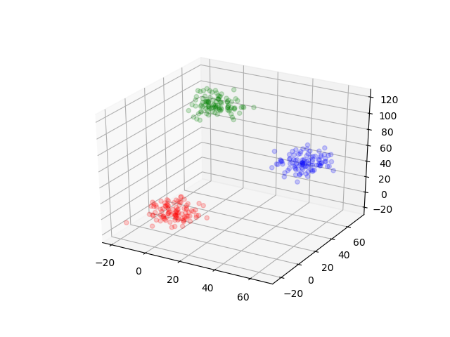

To visualize the outcome.

resultsThree = EM(dataThree, 3)
simpleResultsThree = [argMax(pos) for pos in resultsThree.posterior[end]]
groupOneIndexThree = find(simpleResultsThree .== 1)
groupTwoIndexThree = find(simpleResultsThree .== 2)
groupThreeIndexThree = find(simpleResultsThree .== 3)

scatter3D(dataThree[groupOneIndexThree, 1], dataThree[groupOneIndexThree, 2], dataThree[groupOneIndexThree, 3], color="blue", alpha=0.2)
scatter3D(dataThree[groupTwoIndexThree, 1], dataThree[groupTwoIndexThree, 2], dataThree[groupTwoIndexThree, 3], color="red", alpha=0.2)
scatter3D(dataThree[groupThreeIndexThree, 1], dataThree[groupThreeIndexThree, 2], dataThree[groupThreeIndexThree, 3], color="green", alpha=0.2)
scatter3D(resultsThree.mu[end][1][1], resultsThree.mu[end][1][2], resultsThree.mu[end][1][3], color="black")
scatter3D(resultsThree.mu[end][2][1], resultsThree.mu[end][2][2], resultsThree.mu[end][2][3], color="black")
scatter3D(resultsThree.mu[end][3][1], resultsThree.mu[end][3][2], resultsThree.mu[end][3][3], color="black")

To this data, as before, we can see how the algorithm worked.

function plotThreeDOne(data, results)
    for i in 1:length(results.posterior)
        simpleResults = [argMax(pos) for pos in results.posterior[i]]
        groupOneIndex = find(simpleResults .== 1)
        groupTwoIndex = find(simpleResults .== 2)
        groupThreeIndex = find(simpleResults .== 3)
        figure()
        scatter3D(data[groupOneIndex, 1], data[groupOneIndex, 2], data[groupOneIndex, 3], color="blue", alpha=0.2)
        scatter3D(data[groupTwoIndex, 1], data[groupTwoIndex, 2], data[groupTwoIndex, 3], color="red", alpha=0.2)
        scatter3D(data[groupThreeIndex, 1], data[groupThreeIndex, 2], data[groupThreeIndex, 3], color="green", alpha=0.2)
        scatter3D(results.mu[i][1][1], results.mu[i][1][2], results.mu[i][1][3], color="black")
        scatter3D(results.mu[i][2][1], results.mu[i][2][2], results.mu[i][2][3], color="black")
        scatter3D(results.mu[i][3][1], results.mu[i][3][2], results.mu[i][3][3], color="black")
        savefig("three_d_one_" * string(i) * ".png")
    end
end
plotThreeDOne(dataThree, resultsThree)