Abstract
On this article, I'll try simple regression and classification with Flux, one of the deep learning packages of Julia.Flux
Flux is one of the deep learning packages. When we tackle with deep learning task, we have some choices about libraries. This time, because I read the reddit's post, Julia and “deep learning” and Flux sounded great, I'll touch Flux as a trial.About the detail of Flux, I recommend that you read the official document. Actually, same as Keras's document, the document is very informative and helpful even to grasp the basis of deep learning itself.
GitHub
Official document
Regression
As a first step, I'll do simple regression to the artificial data. The following code is to make the simple artificial data.using Distributions
srand(59)
regX = rand(100)
regY = 100 * regX + rand(Normal(0, 10), 100)
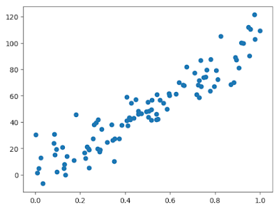
By visualizing, we can grasp the data.
using PyPlot

scatter(regX, regY)

The purpose of the regression is to get the coefficient, meaning 100 here.
Before making the model, I need to adjust the form of data to Flux. As a matter of fact, my research to Flux is not enough. So, it is possible that there is more efficient way.
regData = []
for i in 1:length(regX)
    push!(regData, (regX[i], regY[i]))
end
By Flux, it is easy to build model and train it. Here, I'll define model, loss and optimizer. And the model is trained with the data. If you are already familiar with TensorFlow and Keras, I think you can feel that the Flux code is so friendly.
using Flux
using Flux: @epochs

modelReg = Chain(Dense(1, 1), identity)
loss(x, y) = Flux.mse(modelReg(x), y)
opt = SGD(Flux.params(modelReg), 0.1)
@epochs 100 Flux.train!(loss, regData, opt)
By this, the model was trained to the data with 100 epochs. On this case, the variable, modelReg, contains the trained weight. If test data are given to the model, we can get the predicted values.
predX = linspace(0, 1)
predY = modelReg(predX').data
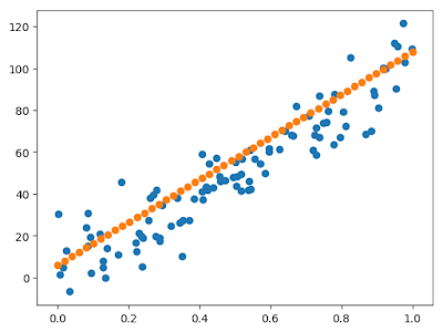
To check the model and prediction visually, we can plot those. It's working well.
scatter(regX, regY)
scatter(predX, predY)

Just in case, by Flux's function, let's check the parameters.
println(Flux.params(modelReg))Any[param([102.043]), param([5.90741])]Those are more or less correct.
Classification
Next, classification. The following code is to make the train and test data.using Distributions
srand(59)
function makeData()
groupOne = rand(MvNormal([10.0, 10.0], 10.0 * eye(2)), 100)
groupTwo = rand(MvNormal([0.0, 0.0], 10 * eye(2)), 100)
groupThree = rand(MvNormal([15.0, 0.0], 10.0 * eye(2)), 100)
return hcat(groupOne, groupTwo, groupThree)'
end
x = makeData()
xTest = makeData()
y = []
for i in 1:300
if 1 <= i <= 100
push!(y, [1, 0, 0])
elseif 101 <= i <= 200
push!(y, [0, 1, 0])
else
push!(y, [0, 0, 1])
end
end
clusterData = []
for i in 1:length(y)
push!(clusterData, (x[i, :], y[i]))
end
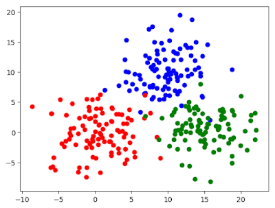
By visualizing those, we can see the data are composed of three clusters. The purpose is to make model to classify.
scatter(x[1:100, 1], x[1:100, 2], color="blue")
scatter(x[101:200, 1], x[101:200, 2], color="red")
scatter(x[201:300, 1], x[201:300, 2], color="green")
With same manner as regression case, we can make the model. The model structure is bit more complex than the regression’s one. On the output layer, the softmax function is used. Also, as a loss function, it is adapting crossentropy.
modelClassify = Chain(Dense(2, 5),
    Dense(5, 3),
    softmax)
loss(x, y) = Flux.crossentropy(modelClassify(x), y)
opt = SGD(Flux.params(modelClassify), 0.01)
@epochs 100 Flux.train!(loss, clusterData, opt)
To the test data, the code below does prediction and checks the accuracy.
predicted = modelClassify(xTest').data
predictedMax = []
for i in 1:size(predicted)[2]
    push!(predictedMax, indmax(predicted[:, i]))
end
println(sum(indmax.(y) .== predictedMax)/300)
0.8333333333333334