Abstract
On this article, I'll write K-medoids with Julia from scratch.Although K-medoids is not so popular algorithm if you compare with K-means, this is simple and strong clustering method like K-means. So, here, as an introduction, I'll show the theory of K-medoids and write it with Julia.
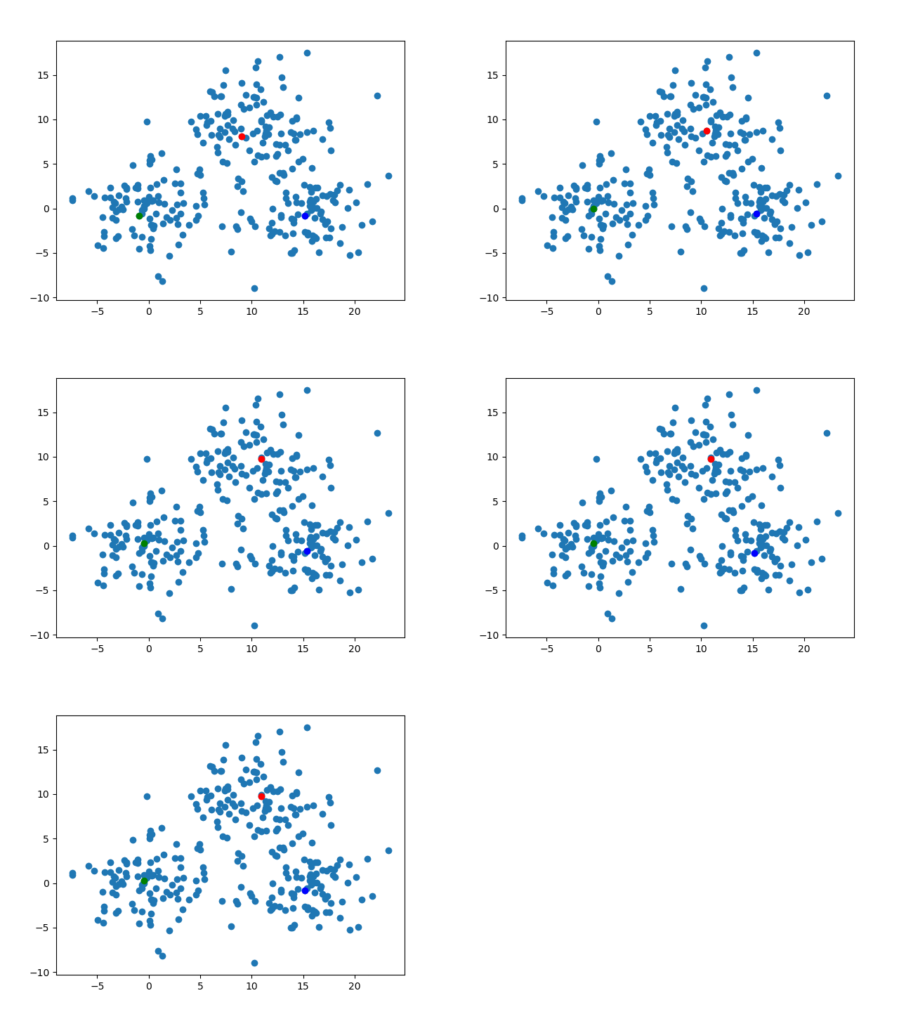
As a goal, I'll make animation like below.
K-medoids
K-medoids is one of the clustering algorithms. It doesn't need label data. Basically, the algorithm is quite similar to K-means algorithm. If you don't know K-means algorithm, please check the article below.K-medoids algorithm is very simple and intuitive. You choose the number, k, of clusters. From the data, randomly choose the k data points as medoids. Each data point belongs to the nearest medoid. In the group(cluster), choose the new medoid. Until it reaches convergence, the updating of medoid and data’s belonging repeats. The different point from K-means algorithm is the medoids. On K-means, the centroid point which corresponds to medoid in K-medoids is a mean of the data points which belong to that corresponding cluster. On K-medoids, the medoids are chosen from the data points which belong to the corresponding cluster.
By arranging, let's check more precisely.
- Initialization
- Update data points belonging
- Update medoids
Initialization
On K-medoids algorithm, the initialization is to choose medoids of clusters. To say more concretely, from the data points, randomly choose k points(the k is the number of the cluster). This is done just one time at first.Update data points belonging
Each data point belongs to the nearest medoid. So, the update data points belonging is to make the data points belong to the nearest medoid.Update medoids
After every data point belong to the nearest medoid, K-medoids chooses new medoids. The rule is simple. Suppose we think about the cluster . The cluster 's medoid is chosen from the data points which belong to the cluster . The rule is that when in the cluster , the sum of distance from other data points is the smallest, that data point is the new medoid.Code
For the simplicity as blog article, I don't extract the code for function responding to the role, meaning the algorithm starts to the end just in one function. Also, although I wrote “from scratch”, to focus on the K-medoids algorithm writing, DataFrames package will be used.Anyway from here, I’ll start to tackle. At first, import the DataFrames package and write composite type. This composite type, kMedoidsResults, will be literally used to store the outcomes of the K-medoids algorithm.
Roughly, the named fields mean as followings.
- x: the clustering target data
- k: the number of the clusters
- medoids: the array which contains the indices of medoids on each step
- groupInfo: the array which contains information of the data point’s belonging to the group on each step
- iterCount: the number of iteration to convergence
using DataFrames

type kMedoidsResults
    x
    k::Int
    medoids::Array{Array}
    groupInfo::Array{Array}
    iterCount::Int
end
The following function, kMedoids(), is the function for K-medoids algorithm. Simply, it has four steps, initialization, updating of group belonging, updating medoids and convergence judgement. Later, I'll explain those four separately.
This function receives distance matrix as an argument. On K-medoids algorithm, we need distance information between data points. So, we should think about the timing of calculating that, meaning there are following two timings to calculate.
- make distance matrix at first about every combination between data points
- make distance matrix on the phase of choosing next medoid in the cluster
Anyway, I'll make distance matrix about whole data points at first. It is sometimes said that it is advantage for K-medoids that it doesn't need coordinate information for clustering, although personally I don't get the point of this. So, I'll make the function receive distance matrix as an argument.
function kMedoids(distanceMatrix, k)
    # initialize
    dataPointsNum = size(distanceMatrix)[1]
    medoidsIndices = shuffle(1:dataPointsNum)[1:k]

    iterCount = 0
    groupInfo = []
    medoids = []
    while true
        # update group belongings
        dataRepresentativeDistances = distanceMatrix[medoidsIndices, :]

        updatedGroupInfo = Array{Int}(size(dataRepresentativeDistances)[2])
        for i in 1:size(dataRepresentativeDistances)[2]
            updatedGroupInfo[i] = sortperm(dataRepresentativeDistances[:, i])[1]
        end
        push!(groupInfo, updatedGroupInfo)

        # update medoids
        updatedMedoids = Array{Int}(k)
        for class in 1:k
            classIndex = find(updatedGroupInfo .== class)
            classDistanceMatrix = distanceMatrix[classIndex, classIndex]
            distanceSum = vec(sum(classDistanceMatrix, 2))
            medoidIndex = classIndex[sortperm(distanceSum)[1]]
            updatedMedoids[class] = medoidIndex
        end

        push!(medoids, updatedMedoids)

        if medoidsIndices == updatedMedoids
            iterCount += 1
            break
        end
        medoidsIndices = updatedMedoids
        iterCount += 1
    end
    return kMedoidsResults(distanceMatrix, k, medoids, groupInfo, iterCount)
end
The code above is bit long and confusing. I'll separate this into four parts corresponding to the role.
The first is the initialization. To say precisely, it is the initialization about the medoids point. On K-medoids algorithm, the medoids are chosen from the data points themselves. Here, I couldn’t find non-overlapping sampling function on Julia. So, I shuffled the data point’s index and extract first k points. These are the indices of data which are chosen as medoids.
    # initialize
    dataPointsNum = size(distanceMatrix)[1]
    medoidsIndices = shuffle(1:dataPointsNum)[1:k]
Second, updating of group belonging. On K-medoids algorithm, any data points belong to a cluster on each iteration. The belonging rule is very simple. Each data points belong to the nearest medoid. The function already has distance matrix. So only thing we need to do is to reference the row or column corresponding to the medoids and check the nearest medoid.
        # update group belongings
        dataRepresentativeDistances = distanceMatrix[medoidsIndices, :]

        updatedGroupInfo = Array{Int}(size(dataRepresentativeDistances)[2])
        for i in 1:size(dataRepresentativeDistances)[2]
            updatedGroupInfo[i] = sortperm(dataRepresentativeDistances[:, i])[1]
        end
        push!(groupInfo, updatedGroupInfo)
Next, we need to update the medoids information based on the information of updated data belonging information. The rule to update the medoids is distance-based. When it updates the cluster 's medoid, it, at first, gets sub-matrix of the original distance matrix on the rule that the data points belong to the cluster . The data point whose sum of distances from other data points in the cluster is the smallest is the updated medoid of the cluster.
        # update medoids
        updatedMedoids = Array{Int}(k)
        for class in 1:k
            classIndex = find(updatedGroupInfo .== class)
            classDistanceMatrix = distanceMatrix[classIndex, classIndex]
            distanceSum = vec(sum(classDistanceMatrix, 2))
            medoidIndex = classIndex[sortperm(distanceSum)[1]]
            updatedMedoids[class] = medoidIndex
        end

        push!(medoids, updatedMedoids)
Same as K-means, the algorithm includes convergence judgement. Here, as a convergence judgement, I set that if the medoids don't change at all, the update loop stops.
        if medoidsIndices == updatedMedoids
            iterCount += 1
            break
        end
Execute
To the artificial data, I'll try the K-medoid.I'll use the artificial data which has two explaining variables. This data will be generated by three types of multivariate normal distributions, meaning we can hope the points should be cleanly classified into three groups.
To show the behavior, I'll visualize it.
using Distributions
using PyPlot
import Distances

function makeData()
    srand(1234)
    groupOne = rand(MvNormal([10.0, 10.0], 10.0 * eye(2)), 100)
    groupTwo = rand(MvNormal([0.0, 0.0], 10 * eye(2)), 100)
    groupThree = rand(MvNormal([15.0, 0.0], 10.0 * eye(2)), 100)
    return hcat(groupOne, groupTwo, groupThree)'
end

data = makeData()
scatter(data[1:100, 1], data[1:100, 2], color="blue")
scatter(data[101:200, 1], data[101:200, 2], color="red")
scatter(data[201:300, 1], data[201:300, 2], color="green")
As you can see, there are three groups.
The purpose of K-medoids execution is to classify these.
As a preparation, we need to choose the number of clusters and make distance matrix. Here, I'll set and by Distances.pairwise() function, make the distance matrix.
kMedoids() function returns kMedoidsResults. kMedoidsResults has the field, groupInfo. This is the predicted classes. It has all the information about group belonging of data points on every iteration. So, the result we want is the last item of the array.(Honestly, this is just confusing. I'm regretting.)
k = 3
distanceMatrix = Distances.pairwise(Distances.SqEuclidean(), data')

results = kMedoids(distanceMatrix, k)
predictedClass = results.groupInfo[size(results.groupInfo)[1]]
To check the outcome, I'll visualize it with the original data. We can see the clustering was done well.
classOneIndex = find(predictedClass .== 1)
classTwoIndex = find(predictedClass .== 2)
classThreeIndex = find(predictedClass .== 3)

subplot(1,2,1)
title("data class")
scatter(data[1:100, 1], data[1:100, 2], color="blue")
scatter(data[101:200, 1], data[101:200, 2], color="red")
scatter(data[201:300, 1], data[201:300, 2], color="green")

subplot(1,2,2)
title("predicted class")
scatter(data[classOneIndex, 1], data[classOneIndex, 2], color="blue")
scatter(data[classTwoIndex, 1], data[classTwoIndex, 2], color="red")
scatter(data[classThreeIndex, 1], data[classThreeIndex, 2], color="green")
Visualize
The kMedoidsResults contains the field which has the information of medoids. To say precisely, those are the medoid's indices on each iteration. We can visualize those easily. By the code below, I'll export the image about the position of the medoids on each steps. The animation gif shows how those move.for (i, medoid) in enumerate(results.medoids)
figure()
scatter(data[:, 1], data[:, 2])
scatter(data[medoid[1], 1], data[medoid[1], 2], color="blue")
scatter(data[medoid[2], 1], data[medoid[2], 2], color="red")
scatter(data[medoid[3], 1], data[medoid[3], 2], color="green")
savefig("medoid_" * string(i) * ".png")
end
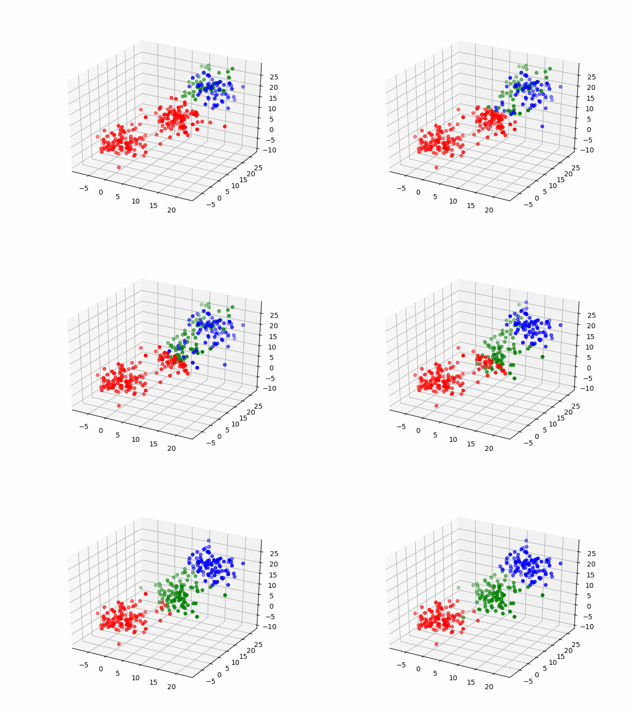
Also, kMedoidsResults has the field for group belonging information on each iteration. I'll make an animation on the same manner.
for (i, group) in enumerate(results.groupInfo)
    classOneIndices = find(group .== 1)
    classTwoIndices = find(group .== 2)
    classThreeIndices = find(group .== 3)

    figure()
    scatter(data[classOneIndices, 1], data[classOneIndices, 2], color="blue")
    scatter(data[classTwoIndices, 1], data[classTwoIndices, 2], color="red")
    scatter(data[classThreeIndices, 1], data[classThreeIndices, 2], color="green")
    savefig("group_" * string(i) * ".png")
end
Next, by the three-dimensional data, I'll do same thing. The data have three groups and by visualization, it becomes as following.
function makeData3D()
    groupOne = rand(MvNormal([10.0, 10.0, 10.0], 10.0 * eye(3)), 100)
    groupTwo = rand(MvNormal([0.0, 0.0, 0.0], 10 * eye(3)), 100)
    groupThree = rand(MvNormal([15.0, 20.0, 20.0], 10.0 * eye(3)), 100)
    return hcat(groupOne, groupTwo, groupThree)'
end

ThreeDimensionsData = makeData3D()

scatter3D(ThreeDimensionsData[1:100,1], ThreeDimensionsData[1:100,2], ThreeDimensionsData[1:100,3], color="red")
scatter3D(ThreeDimensionsData[101:200,1], ThreeDimensionsData[101:200,2], ThreeDimensionsData[101:200,3], color="blue")
scatter3D(ThreeDimensionsData[201:300,1], ThreeDimensionsData[201:300,2], ThreeDimensionsData[201:300,3], color="green")
To the three-dimensional data, I can use kMedoids() function as the same way.
k = 3
distanceMatrixThree = Distances.pairwise(Distances.SqEuclidean(), ThreeDimensionsData')

resultsThree = kMedoids(distanceMatrixThree, k)
The variable, resultsThree, contains medoids and group information on each iteration. At first, I'll visualize how medoids changed in the loop. You can see that as the iteration goes, the medoids move.
for (i, medoid) in enumerate(resultsThree.medoids)
    figure()
    scatter3D(ThreeDimensionsData[:, 1], ThreeDimensionsData[:, 2], ThreeDimensionsData[:, 3], alpha=0.2)
    scatter3D(ThreeDimensionsData[medoid[1], 1], ThreeDimensionsData[medoid[1], 2], ThreeDimensionsData[medoid[1], 3], color="blue")
    scatter3D(ThreeDimensionsData[medoid[2], 1], ThreeDimensionsData[medoid[2], 2], ThreeDimensionsData[medoid[2], 3], color="red")
    scatter3D(ThreeDimensionsData[medoid[3], 1], ThreeDimensionsData[medoid[3], 2], ThreeDimensionsData[medoid[3], 3], color="green")
    savefig("medoid_three_" * string(i) * ".png")
end
Next, group belongings.
for (i, group) in enumerate(resultsThree.groupInfo)
    classOneIndices = find(group .== 1)
    classTwoIndices = find(group .== 2)
    classThreeIndices = find(group .== 3)

    figure()
    scatter3D(ThreeDimensionsData[classOneIndices, 1], ThreeDimensionsData[classOneIndices, 2], ThreeDimensionsData[classOneIndices, 3], color="blue")
    scatter3D(ThreeDimensionsData[classTwoIndices, 1], ThreeDimensionsData[classTwoIndices, 2], ThreeDimensionsData[classTwoIndices, 3], color="red")
    scatter3D(ThreeDimensionsData[classThreeIndices, 1], ThreeDimensionsData[classThreeIndices, 2], ThreeDimensionsData[classThreeIndices, 2], color="green")
    savefig("group_three_" * string(i) * ".png")
end
