Data Science Struggle: Introduction to K-means: Algorithm and Visualization with Julia from scratch

Abstract

On this article, I'll write K-means with Julia from scratch and show animation to see how the algorithm works.
K-means is very simple unsupervised algorithm for clustering. So, when I start to study new programming language, I always use K-means as the theme for writing from scratch.
The following GIF shows how data points are classified into clusters on the way of algorithm going. Relatively easily, we can write K-means code and plot this kind of animation with Julia.

enter image description here

On this article, I used Julia with version 0.6.2.

K-means algorithm

Practically, K-means is used when the following conditions are fulfilled.

You want to do clustering.
The data don’t have label information.

The rule can be expressed as below.
$\mu_k$ : the representative point of cluster k
The cost function is the following $J$ . This contains the optimization of $\mu_k$ and $\tau_{nk}$ .
$J = \sum_{n=1}^{N}\sum_{k=1}^{K} \tau_{nk} ||x_n - \mu_k||^2$
$\tau_{nk} = \begin{eqnarray}\left\{\begin{array}{l} 1 \space if \space k = arg min_j ||x_n - \mu_j||^2\\0 \space otherwise\end{array}\right.\end{eqnarray}$
This optimization can be attained by the following steps.

Initialization
Optimization of representative points
Optimization of data points belonging

Initialization is done only once at first. The optimization of representative points and data points belongings repeat until the data points belongings become stable.

Initialization

As a premise, we assume that there are N data points and K clusters. On initialization phase, we randomly assign the cluster on the data points. To say precisely, we randomly assign cluster k ( $k \in 1,..,K$ ) on data n ( $n \in 1,..,N$ ).

Optimization of representative points

On the K-means algorithm, every cluster has its own representative point. The representative points are calculated as the mean of the data points which belong to the equivalent cluster.

Optimization of data points belonging

Every data point belongs to one cluster. The cluster which one specific data point belongs to depends on the distance between the representative points and the data point. The data point belongs to the nearest representative point.

Code

At first, I'll load necessary packages and make data. The data consist of three groups which have different means and their dimensions are two.

using DataFrames
using Distributions
using PyPlot

function makeData()
    groupOne = rand(MvNormal([10.0, 10.0], 10.0 * eye(2)), 100)
    groupTwo = rand(MvNormal([0.0, 0.0], 10 * eye(2)), 100)
    groupThree = rand(MvNormal([15.0, 0.0], 10.0 * eye(2)), 100)
    return hcat(groupOne, groupTwo, groupThree)'
end

By visualizing, we can see there are three different groups.

data = makeData()
scatter(data[1:100, 1], data[1:100, 2], color="blue")
scatter(data[101:200, 1], data[101:200, 2], color="red")
scatter(data[201:300, 1], data[201:300, 2], color="green")

The main purpose of this article is to make K-means algorithm.
From here, I'll start to tackle with algorithm part. Here, I'll make the kMeans type for the data and nearest k points information.

using StatsBase

type kMeans
    x::DataFrames.DataFrame
    k::Int
end

K-means needs distance calculation. I adopted euclidean distance. Just as an example, I will also write minkowski distance. But this time, only euclidean will be used.

function euclidean(sourcePoint, destPoint)
    sum = 0
    for i in 1:length(sourcePoint)
        sum += (destPoint[i] - sourcePoint[i]) ^ 2
    end
    dist = sqrt(sum)
    return dist
end

function minkowski(sourcePoint, destPoint)
    sum = 0
    for i in 1:length(sourcePoint)
        sum += abs(destPoint[i] - sourcePoint[i])
    end
    return sum
end

function calcDist(sourcePoint::Array, destPoint::Array; method="euclidean")

    if length(sourcePoint) != length(destPoint)
        error("The lengths of two arrays are different.")
        return
    end

    if method == "euclidean"
        return euclidean(sourcePoint, destPoint)
    elseif method == "minkowski"
        return minkowski(sourcePoint, destPoint)
    end
end

The following code is the concrete algorithm part. The function can be separated into three parts, meaning initialization, updating representative points of clusters and updating the data points belongings. On the initialization part, the classes are randomly assigned on the data points. The representative points of clusters are updated by the data points which belong to the equivalent cluster. And after that, the update of data point's belongings is done. Concretely, the distances between data points and the group representative points are calculated and the data point belongs to the cluster whose representative point is the nearest from the data point. To be added, stop decision is also one of the points.

function classify(kMeans::kMeans)
    dataPointsNum = size(kMeans.x, 1)
    estimatedClass = Array{Int}(dataPointsNum)
    sample!(1:kMeans.k, estimatedClass)

    while true
        # update representative points
        representativePoints = []
        for representativeIndex in 1:kMeans.k
            groupIndex = find(estimatedClass .== representativeIndex)
            groupData = kMeans.x[groupIndex, :]

            # TODO: check the return type of colwise
            representativePoint = [ valArray[1] for valArray in colwise(mean, groupData) ]
            push!(representativePoints, representativePoint)
        end

        # update group belonging
        tempEstimatedClass = Array{Int}(dataPointsNum)
        for dataIndex in 1:dataPointsNum
            dataPoint = Array(kMeans.x[dataIndex, :])
            distances = Array{Float64}(kMeans.k)
            for representativeIndex in 1:kMeans.k
                distances[representativeIndex] = calcDist(dataPoint, representativePoints[representativeIndex])
            end

            # TODO: check the existence of argmin
            tempEstimatedClass[dataIndex] = sortperm(distances)[1]
        end

        if estimatedClass == tempEstimatedClass
            break
        end
        estimatedClass = tempEstimatedClass
    end
    return estimatedClass
end

Because the function is bit long, I'll separate this into initialization, update of representative points, update of data points belonging and stop decision.

Initialization

On the initialization part, it made an empty array and randomly assigned cluster on data points. On the following case, sample!() destructively assigned the number ranging from 1 to kMeans.k on array’s factor.

    dataPointsNum = size(kMeans.x, 1)
    estimatedClass = Array{Int}(dataPointsNum)
    sample!(1:kMeans.k, estimatedClass)

Update of representative points

Every data points has its belonging to specific cluster. The cluster member's mean will be the updated representative point of the cluster.
On the following code, find() function is equivalent to numpy's where() method on Python, meaning it returns the index when the value fulfills the condition. By colwise() function, we can get the mean value based on columns.

        # update representative points
        representativePoints = []
        for representativeIndex in 1:kMeans.k
            groupIndex = find(estimatedClass .== representativeIndex)
            groupData = kMeans.x[groupIndex, :]

            representativePoint = [ valArray[1] for valArray in colwise(mean, groupData) ]
            push!(representativePoints, representativePoint)
        end

Update of data points belonging

Here, the following code is to update data points belonging. The system is very simple. The distances between specific data point and cluster's representative points are calculated and the data point belongs to the nearest representative point.

        # update group belonging
        tempEstimatedClass = Array{Int}(dataPointsNum)
        for dataIndex in 1:dataPointsNum
            dataPoint = Array(kMeans.x[dataIndex, :])
            distances = Array{Float64}(kMeans.k)
            for representativeIndex in 1:kMeans.k
                distances[representativeIndex] = calcDist(dataPoint, representativePoints[representativeIndex])
            end

            # TODO: check the existence of argmin
            tempEstimatedClass[dataIndex] = sortperm(distances)[1]
        end

Stop decision

This time, as a stop judgement, I set the rule that if the data belonging doesn't change at all in the loop, it stops.

        if estimatedClass == tempEstimatedClass
            break
        end

Execute and Visualize

The naive K-means algorithm was written. By two lines, we can execute that.

kmeans = kMeans(DataFrame(data), 3)
predictedClass = classify(kmeans)

This time I'll skip the evaluation phase and just do visualization. To compare with real class, I show the real class plot and the predicted class plot at once.

classOneIndex = find(predictedClass .== 1)
classTwoIndex = find(predictedClass .== 2)
classThreeIndex = find(predictedClass .== 3)

subplot(1,2,1)
title("data class")
scatter(data[1:100, 1], data[1:100, 2], color="blue")
scatter(data[101:200, 1], data[101:200, 2], color="red")
scatter(data[201:300, 1], data[201:300, 2], color="green")

subplot(1,2,2)
title("predicted class")
scatter(data[classOneIndex, 1], data[classOneIndex, 2], color="blue")
scatter(data[classTwoIndex, 1], data[classTwoIndex, 2], color="red")
scatter(data[classThreeIndex, 1], data[classThreeIndex, 2], color="green")

As you can see, the data points are well classified.
Next, to deepen the insight into K-means algorithm, I'll visualize how the representative points move and the data point's belonging changes.
By adding some lines to the classify() function, I'll make the classify() function write out the plot in every iteration to know how the representative points move and the data belongings change. The function below is hard-coded to the data's dimension.

function classifyViz(kMeans::kMeans)
    dataPointsNum = size(kMeans.x, 1)
    estimatedClass = Array{Int}(dataPointsNum)
    sample!(1:kMeans.k, estimatedClass)

    i = 1
    while true
        # update representative points
        representativePoints = []
        for representativeIndex in 1:kMeans.k
            groupIndex = find(estimatedClass .== representativeIndex)
            groupData = kMeans.x[groupIndex, :]

            # TODO: check the return type of colwise
            representativePoint = [ valArray[1] for valArray in colwise(mean, groupData) ]
            push!(representativePoints, representativePoint)
        end

        # visualize
        figure()
        scatter(Array(kMeans.x[:,1]), Array(kMeans.x[:,2]))
        scatter(representativePoints[1][1], representativePoints[1][2], color="blue")
        scatter(representativePoints[2][1], representativePoints[2][2], color="red")
        scatter(representativePoints[3][1], representativePoints[3][2], color="green")
        savefig("./output/representative_" * string(i) * ".png")

        # visualize
        figure()
        scatter(Array(kMeans.x[:,1]), Array(kMeans.x[:,2]))
        groupOneInd = find(estimatedClass .== 1)
        groupTwoInd = find(estimatedClass .== 2)
        groupThreeInd = find(estimatedClass .== 3)
        scatter(Array(kMeans.x[groupOneInd,1]), Array(kMeans.x[groupOneInd,2]), color="blue")
        scatter(Array(kMeans.x[groupTwoInd,1]), Array(kMeans.x[groupTwoInd,2]), color="red")
        scatter(Array(kMeans.x[groupThreeInd,1]), Array(kMeans.x[groupThreeInd,2]), color="green")
        savefig("./output/data_" * string(i) * ".png")

        # update group belonging
        tempEstimatedClass = Array{Int}(dataPointsNum)
        for dataIndex in 1:dataPointsNum
            dataPoint = Array(kMeans.x[dataIndex, :])
            distances = Array{Float64}(kMeans.k)
            for representativeIndex in 1:kMeans.k
                distances[representativeIndex] = calcDist(dataPoint, representativePoints[representativeIndex])
            end

            # TODO: check the existence of argmin
            tempEstimatedClass[dataIndex] = sortperm(distances)[1]
        end

        i += 1

        if estimatedClass == tempEstimatedClass
            break
        end
        estimatedClass = tempEstimatedClass
    end
    return estimatedClass
end

By executing the function, the plot images are saved.

classifyViz(kmeans)

I made GIF images from the data.

Data belonging

The GIF of data point's belonging is as following. Because this data is relatively easy, after just few iteration, we can see those points are well classified.

enter image description here

Representative points

The GIF below shows how the representative points of clusters move.

enter image description here

Visualize 3D data

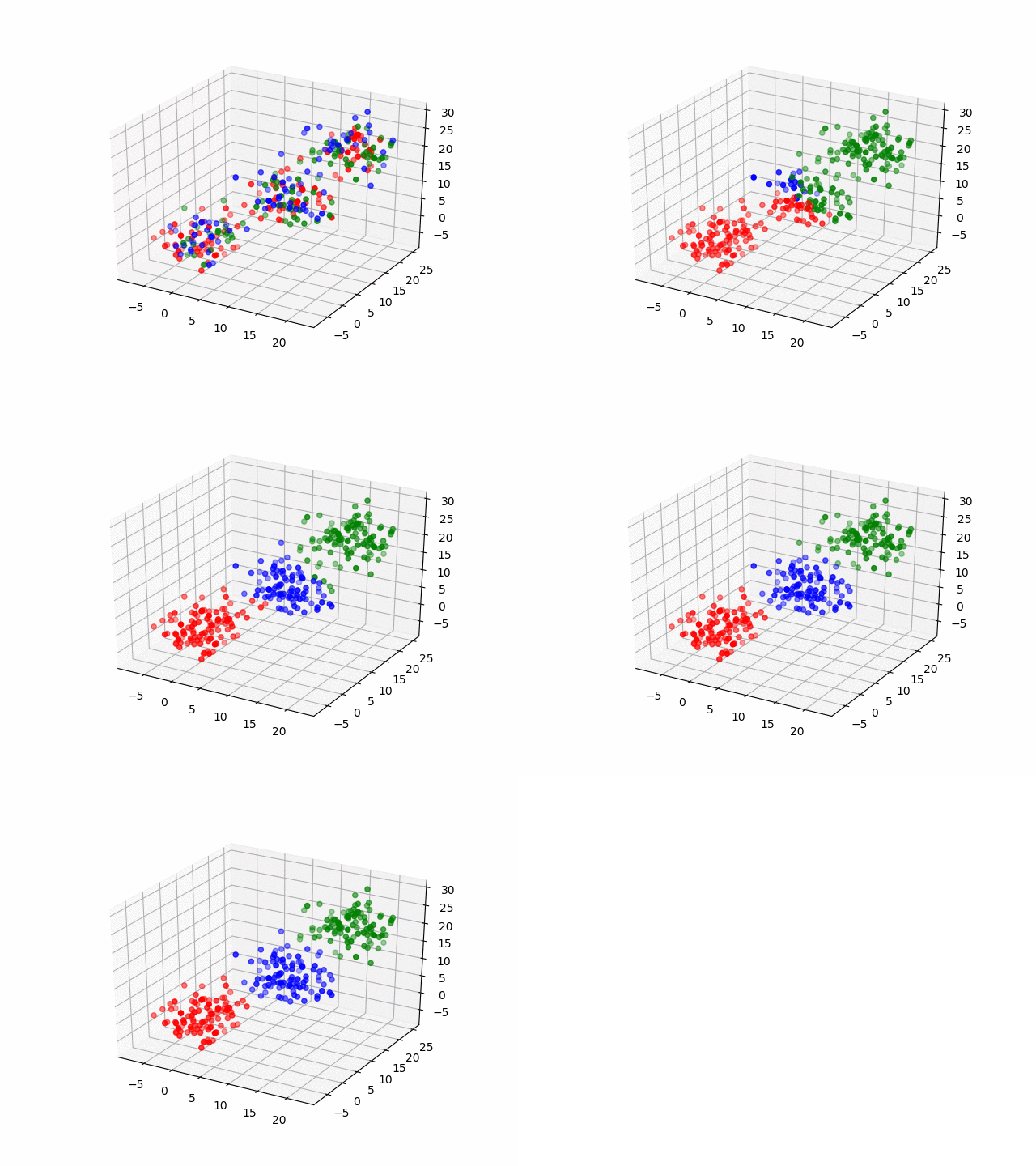
Until here, I wrote K-means algorithm and visualize. The data were composed of two columns and in visualization, the plot was two dimension. Here, from now on, I'll show the case of 3D.
The data are like this.

function makeData3D()
    groupOne = rand(MvNormal([10.0, 10.0, 10.0], 10.0 * eye(3)), 100)
    groupTwo = rand(MvNormal([0.0, 0.0, 0.0], 10 * eye(3)), 100)
    groupThree = rand(MvNormal([15.0, 20.0, 20.0], 10.0 * eye(3)), 100)
    return hcat(groupOne, groupTwo, groupThree)'
end

ThreeDimensionsData = makeData3D()

scatter3D(ThreeDimensionsData[1:100,1], ThreeDimensionsData[1:100,2], ThreeDimensionsData[1:100,3], color="red")
scatter3D(ThreeDimensionsData[101:200,1], ThreeDimensionsData[101:200,2], ThreeDimensionsData[101:200,3], color="blue")
scatter3D(ThreeDimensionsData[201:300,1], ThreeDimensionsData[201:300,2], ThreeDimensionsData[201:300,3], color="green")

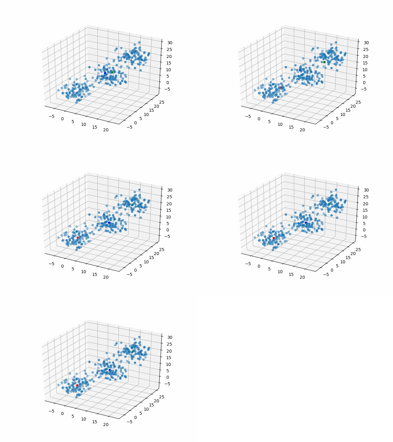
There are three groups. Here, what I'll do is the clustering and visualization. About the visualization, to say precisely, I'm trying to check how data points belonging changes and the representative points move.
Same as the case of 2D, I'll change a bit of the classify() function. For visualization, some lines will be added. The function below will write out the plot image in every iteration to know how the representative points move and the data belongings change.

function classifyViz3D(kMeans::kMeans)
    dataPointsNum = size(kMeans.x, 1)
    estimatedClass = Array{Int}(dataPointsNum)
    sample!(1:kMeans.k, estimatedClass)

    i = 1
    while true
        # update representative points
        representativePoints = []
        for representativeIndex in 1:kMeans.k
            groupIndex = find(estimatedClass .== representativeIndex)
            groupData = kMeans.x[groupIndex, :]

            # TODO: check the return type of colwise
            representativePoint = [ valArray[1] for valArray in colwise(mean, groupData) ]
            push!(representativePoints, representativePoint)
        end

        # visualize
        figure()
        scatter3D(Array(kMeans.x[:,1]), Array(kMeans.x[:,2]), Array(kMeans.x[:,3]))
        scatter3D(representativePoints[1][1], representativePoints[1][2], representativePoints[1][3], color="blue")
        scatter3D(representativePoints[2][1], representativePoints[2][2], representativePoints[2][3], color="red")
        scatter3D(representativePoints[3][1], representativePoints[3][2], representativePoints[3][3], color="green")
        savefig("./output/representative3d_" * string(i) * ".png")

        # visualize
        figure()
        groupOneInd = find(estimatedClass .== 1)
        groupTwoInd = find(estimatedClass .== 2)
        groupThreeInd = find(estimatedClass .== 3)
        scatter3D(Array(kMeans.x[groupOneInd,1]), Array(kMeans.x[groupOneInd,2]), Array(kMeans.x[groupOneInd,3]), color="blue")
        scatter3D(Array(kMeans.x[groupTwoInd,1]), Array(kMeans.x[groupTwoInd,2]), Array(kMeans.x[groupTwoInd,3]), color="red")
        scatter3D(Array(kMeans.x[groupThreeInd,1]), Array(kMeans.x[groupThreeInd,2]), Array(kMeans.x[groupThreeInd,3]), color="green")
        savefig("./output/data3d_" * string(i) * ".png")

        # update group belonging
        tempEstimatedClass = Array{Int}(dataPointsNum)
        for dataIndex in 1:dataPointsNum
            dataPoint = Array(kMeans.x[dataIndex, :])
            distances = Array{Float64}(kMeans.k)
            for representativeIndex in 1:kMeans.k
                distances[representativeIndex] = calcDist(dataPoint, representativePoints[representativeIndex])
            end

            # TODO: check the existence of argmin
            tempEstimatedClass[dataIndex] = sortperm(distances)[1]
        end

        i += 1

        if estimatedClass == tempEstimatedClass
            break
        end
        estimatedClass = tempEstimatedClass
    end
    return estimatedClass
end

By the exported images, I made GIF images.

Data belonging

In 3D space, we can see how data point's belonging change in the loop.

enter image description here

Representative points

Also, the representative points of the clusters move as following.

enter image description here

Try Iris data

As an appendix, I'll show visualization of K-means clustering to Iris dataset. On Julia, we can load Iris dataset from RDatasets package.

using RDatasets
iris = dataset("datasets", "iris")

This dataset has four explaining variables and class information. Here, for 3-dimensional visualization, I'll just use three of those explaining variables. Concretely, the variables, SepalLength, SepalWidth and PetalLength, are used for clustering.
The code blow is to visualize the data with those three variables. The colors mean the class information.

setosaIndex = find(Array(iris[:, [:Species]]) .== "setosa")
versicolorIndex = find(Array(iris[:, [:Species]]) .== "versicolor")
virginicaIndex = find(Array(iris[:, [:Species]]) .== "virginica")

scatter3D(Array(iris[setosaIndex, [:SepalLength]]), Array(iris[setosaIndex, [:SepalWidth]]), Array(iris[setosaIndex, [:PetalLength]]), color="red")
scatter3D(Array(iris[versicolorIndex, [:SepalLength]]), Array(iris[versicolorIndex, [:SepalWidth]]), Array(iris[versicolorIndex, [:PetalLength]]), color="blue")
scatter3D(Array(iris[virginicaIndex, [:SepalLength]]), Array(iris[virginicaIndex, [:SepalWidth]]), Array(iris[virginicaIndex, [:PetalLength]]), color="green")

For clustering and visualization, classifyViz3D() function can be used as it is. But, here, just to avoid complexity, I changed the name of image file which will be written out in the loop and also function name.

function classifyViz3DIris(kMeans::kMeans)
    dataPointsNum = size(kMeans.x, 1)
    estimatedClass = Array{Int}(dataPointsNum)
    sample!(1:kMeans.k, estimatedClass)

    i = 1
    while true
        # update representative points
        representativePoints = []
        for representativeIndex in 1:kMeans.k
            groupIndex = find(estimatedClass .== representativeIndex)
            groupData = kMeans.x[groupIndex, :]

            # TODO: check the return type of colwise
            representativePoint = [ valArray[1] for valArray in colwise(mean, groupData) ]
            push!(representativePoints, representativePoint)
        end

        # visualize
        figure()
        scatter3D(Array(kMeans.x[:,1]), Array(kMeans.x[:,2]), Array(kMeans.x[:,3]))
        scatter3D(representativePoints[1][1], representativePoints[1][2], representativePoints[1][3], color="blue")
        scatter3D(representativePoints[2][1], representativePoints[2][2], representativePoints[2][3], color="red")
        scatter3D(representativePoints[3][1], representativePoints[3][2], representativePoints[3][3], color="green")
        savefig("./output/representative3d_iris_" * string(i) * ".png")

        # visualize
        figure()
        groupOneInd = find(estimatedClass .== 1)
        groupTwoInd = find(estimatedClass .== 2)
        groupThreeInd = find(estimatedClass .== 3)
        scatter3D(Array(kMeans.x[groupOneInd,1]), Array(kMeans.x[groupOneInd,2]), Array(kMeans.x[groupOneInd,3]), color="blue")
        scatter3D(Array(kMeans.x[groupTwoInd,1]), Array(kMeans.x[groupTwoInd,2]), Array(kMeans.x[groupTwoInd,3]), color="red")
        scatter3D(Array(kMeans.x[groupThreeInd,1]), Array(kMeans.x[groupThreeInd,2]), Array(kMeans.x[groupThreeInd,3]), color="green")
        savefig("./output/data3d_iris_" * string(i) * ".png")

        # update group belonging
        tempEstimatedClass = Array{Int}(dataPointsNum)
        for dataIndex in 1:dataPointsNum
            dataPoint = Array(kMeans.x[dataIndex, :])
            distances = Array{Float64}(kMeans.k)
            for representativeIndex in 1:kMeans.k
                distances[representativeIndex] = calcDist(dataPoint, representativePoints[representativeIndex])
            end

            # TODO: check the existence of argmin
            tempEstimatedClass[dataIndex] = sortperm(distances)[1]
        end

        i += 1

        if estimatedClass == tempEstimatedClass
            break
        end
        estimatedClass = tempEstimatedClass
    end
    return estimatedClass
end

By executing the following code, the images are written out.

kmeansIris = kMeans(iris[:, [:SepalLength, :SepalWidth, :PetalLength]], 3)
classifyViz3DIris(kmeansIris)

Appendix: How to choose the number of clusters

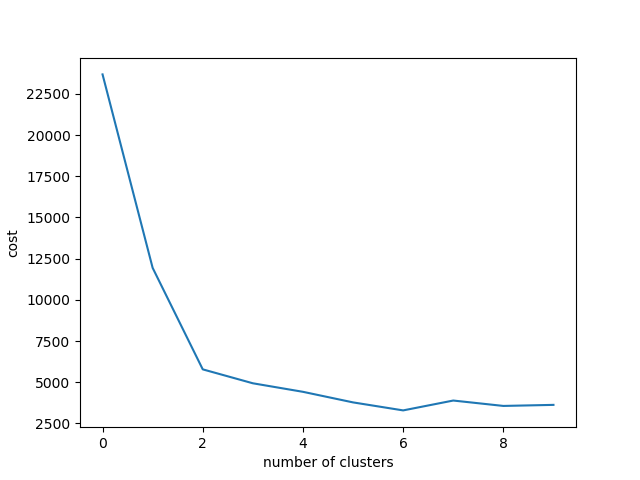
On K-means algorithm, we need to determine the value $k$ , the number of clusters. There are some methods to determine that. Here, I'll show elbow method.
On K-means algorithm, cost function is the following $J$ as I showed before.
$J = \sum_{n=1}^{N}\sum_{k=1}^{K} \tau_{nk} ||x_n - \mu_k||^2$
On elbow method, we calculate the value $J$ on candidate number of clusters and by plotting, we determine the appropriate number of clusters. The point where the degree of tilt changes much is the appropriate number of clusters.
Actually, when I wrote the function, classify(), I didn't think I would show this. So, to save the value $J$ , I adapted bit inefficient way. But it’s not important.
Anyway by the following function, it also return the value of $J$ .

function classifyCost(kMeans::kMeans)
    dataPointsNum = size(kMeans.x, 1)
    estimatedClass = Array{Int}(dataPointsNum)
    sample!(1:kMeans.k, estimatedClass)

    costArray = []
    while true
        # update representative points
        representativePoints = []
        for representativeIndex in 1:kMeans.k
            groupIndex = find(estimatedClass .== representativeIndex)
            groupData = kMeans.x[groupIndex, :]

            # TODO: check the return type of colwise
            representativePoint = [ valArray[1] for valArray in colwise(mean, groupData) ]
            push!(representativePoints, representativePoint)
        end

        # update group belonging
        tempEstimatedClass = Array{Int}(dataPointsNum)

        cost = 0.0
        for dataIndex in 1:dataPointsNum
            dataPoint = Array(kMeans.x[dataIndex, :])
            distances = Array{Float64}(kMeans.k)
            for representativeIndex in 1:kMeans.k
                distances[representativeIndex] = calcDist(dataPoint, representativePoints[representativeIndex])
            end

            # TODO: check the existence of argmin
            classIndex = sortperm(distances)[1]
            tempEstimatedClass[dataIndex] = classIndex
            cost += distances[classIndex] ^ 2

        end
        push!(costArray, cost)

        if estimatedClass == tempEstimatedClass
            break
        end
        estimatedClass = tempEstimatedClass
    end
    return estimatedClass, costArray[length(costArray)]
end

Let's try some number of clusters with the artificial data I made before.

costArray = []
for k in 1:10
    kmeansElbow = kMeans(DataFrame(data), k)
    predictedClassElbow, cost = classifyCost(kmeansElbow)
    push!(costArray, cost)
end

xlabel("number of cluster")
ylabel("cost")
plot(costArray)

As you can see, there are points around two or three, although it is partially controversy to judge. Just in case, by the data which has six classes and the low variance, I'll try.

function makeDataSix()
    srand(59)
    groupOne = rand(MvNormal([10.0, 10.0], 1.0 * eye(2)), 100)
    groupTwo = rand(MvNormal([0.0, 0.0], 1 * eye(2)), 100)
    groupThree = rand(MvNormal([15.0, 0.0], 1.0 * eye(2)), 100)
    groupFour = rand(MvNormal([30.0, 20.0], 1.0 * eye(2)), 100)
    groupFive = rand(MvNormal([0.0, -20.0], 1.0 * eye(2)), 100)
    groupSix = rand(MvNormal([10.0, -50.0], 1.0 * eye(2)), 100)
    return hcat(groupOne, groupTwo, groupThree, groupFour, groupFive, groupSix)'
end

dataSix = makeDataSix()
costArraySix = []
for k in 1:10
    kmeansElbow = kMeans(DataFrame(dataSix), k)
    predictedClassElbow, cost = classifyCost(kmeansElbow)
    push!(costArraySix, cost)
end

xlabel("number of clusters")
ylabel("cost")
plot(costArraySix)

Somehow, it looks like having changing point around six and seven, although personally I feel it has elbow in k=2.

enter image description here

Data Science Struggle

Sunday, April 8, 2018

Introduction to K-means: Algorithm and Visualization with Julia from scratch

Abstract

K-means algorithm

Initialization

Optimization of representative points

Optimization of data points belonging

Code

Initialization

Update of representative points

Update of data points belonging

Stop decision

Execute and Visualize

Data belonging

Representative points

Visualize 3D data

Data belonging

Representative points

Try Iris data

Appendix: How to choose the number of clusters

Reference

Blog Archive