Abstract
This article covers basic understanding and coding of Dense block of DenseNets. DenseNets is one of the convolutional neural network models. If you have an experience of using fine-tuning or frequently tackle with image recognition tasks, probably you have heard that before.DenseNets is composed of Dense blocks. It is expressed as the image below, which is quoted from https://arxiv.org/abs/1608.06993.

On the context of the history of convolutional neural network, ResNet helps the network to be deeper without degradation problem by the shortcut path to the output of the Residual module. DenseNets and Dense block is near concept from the different approach.
This article is to help to understand the basic concept of Dense block of DenseNets and how to write that. For coding, I’ll use Python and Keras.
About the ResNet and Residual module, please read the article below.
If you want to know the detail of DenseNets and Dense block, I recommend you read the article below.
When you find a mistake, please let me know by comment or mail.
Dense block
Structure of Convolutional Neural Network
Before tackling with Dense block, I'll roughly touch the structure of CNN(Convolutional Neural Network) itself. CNN is composed of convolutional layer and dense layer, although to say precisely input, output layers and pooling layers should be added. And about network architecture, we need to care about the number of layers and nodes.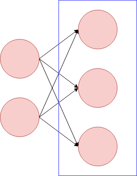
On the image above, the red circles express the nodes. The blue rectangle expresses one layer. When we make CNN model, we need to think about those of convolutional and dense layer.
From here, let’s focus on convolutional layer. Assume there is an image like below. The height and width are four.
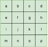
When we adapt convolution to this, we will choose the kernel size. The example below is the kernel with the size (3, 3) with stride (1,1).
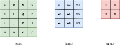
On the context of convolutional neural network, the parameters w1 ~ w9 are the targets to update.
As you can see, by the size of kernel, the outcome of the convolutional network changes.
Dense block
DenseNets is one of the convolutional neural network models. On the context of the state of the art of image classification or fine-tuning, probably you have heard the name of it. Relatively easily, you can try it on Keras.On this article, I'll mention Dense block, which composes DenseNets. The idea is simple and powerful, although in my personal opinion it has some points we need to care about. The Dense block can be expressed by the image below, which is quoted from the thesis, https://arxiv.org/abs/1608.06993.

As you can see, the block is composed of some convolutional layers. From the viewpoint of the structure, the characteristics of the block is the input of each convolutional layers in the block. Each convolutional layer's output will become the inputs of all the following convolutional layers.
To make it simpler, please look at the drawing below. Although this doesn't express Dense block precisely, it works to grasp the point. This Dense block has three convolutional layers. The green arrows from Conv1 to Conv2 and from Conv2 to Conv3 are seen in usual convolutional neural network. The output of Conv1 goes to the input of Conv2 and the output of Conv2 goes to the input of Conv3. The point of Dense block is the brown arrow from the output of Conv1 to the input of Conv3.

We can see this pattern in Residual module. The image below shows Residual module. The input skips some layers and is merged to the output. In Residual module, as it is written like , the input is added to the output.

The image is from https://arxiv.org/abs/1512.03385.
But, the way of being merged in Dense block is different from the one in Residual module. In Dense block, it is by concatenation that the data which skipped layers is merged to the layer's input.
Because of this structural characteristics, DenseNet, which is composed of Dense blocks, can have the following advantages.
- improved flow of information and gradients, making it easy to train the model
- working well with few number of parameters
Each layer has direct access to the gradients from the loss function and the original input signal, leading to an implicit deep supervisionAbout the second one, by catching up with the explanation for now, you may feel strange. The Dense block has some convolutional layers and each layer's output will be merged to the inputs to all the following layers by concatenation. It means that in Dense block, if the layer is located on the later part of the block, the input data size for the layer becomes big. So, we can think that with Dense block, the number of parameters becomes huge. However, actually, it doesn't happen. That's because for DenseNets, it is not necessary to make the layers wide. With this structure, few number of nodes per layer is okay.
Code
With Python and Keras, I'll make a Dense block and train it. This is just a small experiment. So, as a dataset, I'll use MNIST.At first, load the MNIST dataset and do pre-processing. This time, to shorten the time for train, only 2000 data points are used.
from keras.datasets import mnist
from keras.utils import to_categorical

(x_train, y_train), (x_test, y_test) = mnist.load_data()

x_train = x_train.reshape((60000, 28, 28, 1))[0:2000]
y_train = to_categorical(y_train, 10)[0:2000]
As I showed, DenseNets is composed of Dense blocks. And Dense block is composed of some convolutional layer’s blocks. Before making a function for Dense block, I’ll make a function for this convolutional layer’s block. On the image below, it is the part which is surrounded by the black circle.

The image above is from https://arxiv.org/abs/1608.06993. The black circle was added by the writer of this article.
The convolutional block is composed of batch normalization, convolutional layer and Relu function.
from keras.layers import Conv2D, ReLU, BatchNormalization

def dense_factor(inputs):
    h_1 = BatchNormalization()(inputs)
    h_1 = Conv2D(12, (3,3), border_mode='same')(h_1)
    output = ReLU()(h_1)
    return output
Next, by embedding the convolutional block, I'll define Dense block. The purpose of this article is not the exploration into accuracy but to check Dense block itself and how to write it. So, by using the few number of convolutional layers, I'll define the block.
from keras.layers import Input, Flatten, Dense, concatenate
from keras.models import Model
import keras

def dense_block(inputs):

    concatenated_inputs = inputs

    for i in range(3):
        x = dense_factor(concatenated_inputs)
        concatenated_inputs = concatenate([concatenated_inputs, x], axis=3)

    return concatenated_inputs
By using the Dense block, we can make a model. Basically, when we make a model with Dense blocks, we will use some Dense blocks and between them, should set transition layers. But, that is out of range of this article. Therefore, I don't touch it. Just with one Dense block, I'll make a model and train it with MNIST dataset.
def dense_block_model(x_train):
    inputs = Input(x_train.shape[1:])

    x = dense_block(inputs)
    x = Flatten()(x)
    x = Dense(64, activation='softmax')(x)
    predictions = Dense(10, activation='softmax')(x)

    model = Model(input=inputs, output=predictions)

    model.compile(loss=keras.losses.categorical_crossentropy,
                 optimizer=keras.optimizers.SGD(lr=1e-2, decay=1e-6),
                 metrics=['accuracy'])
    return model

model_dense_block = dense_block_model(x_train)
model_dense_block.fit(x_train, y_train, epochs=500, shuffle=True, validation_split=0.1)
We can visualize it by PyPlot.
%matplotlib inline
import matplotlib.pyplot as plt

def show_history(history):
    plt.plot(history.history['acc'])
    plt.plot(history.history['val_acc'])
    plt.ylabel('accuracy')
    plt.xlabel('epoch')
    plt.legend(['train_accuracy', 'validation_accuracy'], loc='best')
    plt.show()

show_history(model_dense_block.history)
