Abstract
This article is to think about the model which is with AUC objective function by some evaluation methods. Also, I can say this is to think about the AUC objective function from the viewpoint of evaluation as the title of the article shows.On the article, AUC as an objective function: with Julia and Optim.jl package, I made a model with AUC objective function. The predicted score by that was distributed in really narrow area, because AUC objective function is based on the order without caring the distance from explained variable. With some evaluation norms, the model's score seems not nice.
About this point, just in case, I'll leave the simple experiment.
Julia: version 0.6.3
Data
This is easy and simple experiment. So, here, I'll use IRIS data set, which is easy to access and many people are used to using.using RDatasets
iris = dataset("datasets", "iris")
# standardization
for col in names(iris)
if col == :Species
continue
end
iris[col] = (iris[col] - mean(iris[col]))/std(iris[col])
end
iris[:Species] = map(x->x=="versicolor"?1:0, Array(iris[:Species]))
The task is to make a model to classify IRIS's versicolor and the others.
To compare
The purpose of this article is to check how good (or bad) the model by AUC objective function is, when you evaluate the model with some evaluation methods. For the comparison, I'll prepare another model with GLM package.using GLM
logit = glm(@formula(Species ~ SepalLength + SepalWidth + PetalLength + PetalWidth), iris, Binomial(), LogitLink())
lrPred = predict(logit, iris[[:SepalLength, :SepalWidth, :PetalLength, :PetalWidth]])
Basically, with good manner, we should split the data into train and test ones. But, here, I don't. With the model trained by whole IRIS data, I did prediction to the same data.
AUC objective function
I'll make a model with naive AUC objective function. About the detail, please check the article below.using Optim
global sepalLength = Array(iris[:SepalLength])
global sepalWidth = Array(iris[:SepalWidth])
global petalLength = Array(iris[:PetalLength])
global petalWidth = Array(iris[:PetalWidth])
global species = Array(iris[:Species])
function objective(w::Array{Float64})
# logistic regression
logistic(t) = (1 + e^(-t))^(-1)
t = w[1] + w[2] * sepalLength + w[3] * sepalWidth + w[4] * petalLength + w[5] * petalWidth
yPred = map(logistic, t)
positiveIndex = find(1 .== species)
negativeIndex = find(0 .== species)
function opt()
s = 0
for pI in positiveIndex
for nI in negativeIndex
if yPred[pI] > yPred[nI]
s += 1
end
end
end
return s
end
return -opt()
end
aucLr = optimize(objective, [0.0, 0.0, 0.0, 0.0, 0.0])
Here, I also made a model with whole IRIS data set and do prediction to the same data.
w = aucLr.minimizer
logistic(t) = (1 + e^(-t))^(-1)
t = w[1] + w[2] * sepalLength + w[3] * sepalWidth + w[4] * petalLength + w[5] * petalWidth
aucPred = map(logistic, t)
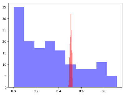
By visualizing the score distribution of those, we can see the difference. We will check what kind of effect this difference has on the phase of evaluation.
using PyPlot

plt[:hist](Float64.(lrPred), color="blue", alpha=0.5)
plt[:hist](aucPred, color="red", alpha=0.5)

Evaluate with some methods
The variables, and , hold the predicted scores. I'll evaluate those with some methods. Here, I'll adapt accuracy, AUC and brier.About AUC and brier, you can use function from the link below.
About accuracy, because the models give scores in the form with the range from 0 to 1, we need to think about the threshold. If I talk about this point, I'll deviate the way of the main theme of this article. So, by trying many thresholds, the highest accuracy will be adapted as “accuracy”, here.
Anyway, to and , I'll evaluate with those evaluation methods.
include("./MLUtils.jl/src/utils.jl")
using MLBase

function accuracy(yTruth::Array{Int}, yPred::Array{Float64})
    accuracies = []
    for i in range(0,0.001,1000)
        yPredInt = map(x->x>=i?1:0, yPred)
        cr = correctrate(yTruth, yPredInt)
        push!(accuracies, cr)
    end
    return maximum(accuracies)
end

@show auc(species, Float64.(lrPred))
@show auc(species, aucPred)
@show brier(species, Float64.(lrPred))
@show brier(species, aucPred)
@show accuracy(species, Float64.(lrPred))
@show accuracy(species, aucPred)
auc(species, Float64.(lrPred)) = 0.8258
auc(species, aucPred) = 0.8312
brier(species, Float64.(lrPred)) = 0.16281623291323666
brier(species, aucPred) = 0.24872485102698297
accuracy(species, Float64.(lrPred)) = 0.7666666666666667
accuracy(species, aucPred) = 0.76
About the accuracy and the AUC scores, there are not big difference. But we can see the difference about brier score.
The brier score is the mean squared error of the forecast in effect. It can be expressed as following. So, about brier score, the lower is better.
- : the score that was forecast
- : the actual outcome of the event
On this case, usual GLM package's model is better than the one with AUC objective function from the viewpoint of brier score. Although, here, I'll avoid the mathematical detail, this outcome matches our intuition. The AUC objective function uses the order of the points which belong to positive and negative. Different from likelihood function, it doesn't use the distance information between the forecast score and the actual outcome.